One of the most persistent confusions in urban research is the assumption that an analytical map is an unfinished presentation map. Under that assumption, the researcher first produces a GIS output containing many layers and then “improves” it for a report by changing colours, hiding a few labels and adding a title. The workflow sounds efficient, but it overlooks an important distinction. Analytical maps and presentation maps are different instruments of reasoning. One helps investigate relationships, test assumptions and detect exceptions. The other communicates a selected result to a defined audience. Neither form is inherently more rigorous; each becomes unreliable when its purpose is misunderstood.
Consider a researcher studying the connection between street-network configuration and pedestrian movement. During analysis, many diagnostic maps may be necessary: network segments, field observations, model outputs, unusual links and areas where the data are incomplete. A published figure cannot necessarily display all of that simultaneously. It must present an interpretable comparison and an explicit claim. Professional cartographic guidance emphasises visual hierarchy and figure-ground organisation as tools for determining which information readers encounter first (Esri cartography guidance); official statistical guidance also advises using a map only when the geographic pattern is central to the argument (ONS choropleth guidance).
The central thesis of this article is that good urban research needs both map types and a documented translation between them. That translation involves changes in selection, visual encoding, annotation, scale and evidential caveats. It should not involve quietly changing the underlying measure to suit the desired visual result.
An analytical map is a workspace for inquiry, testing and revision
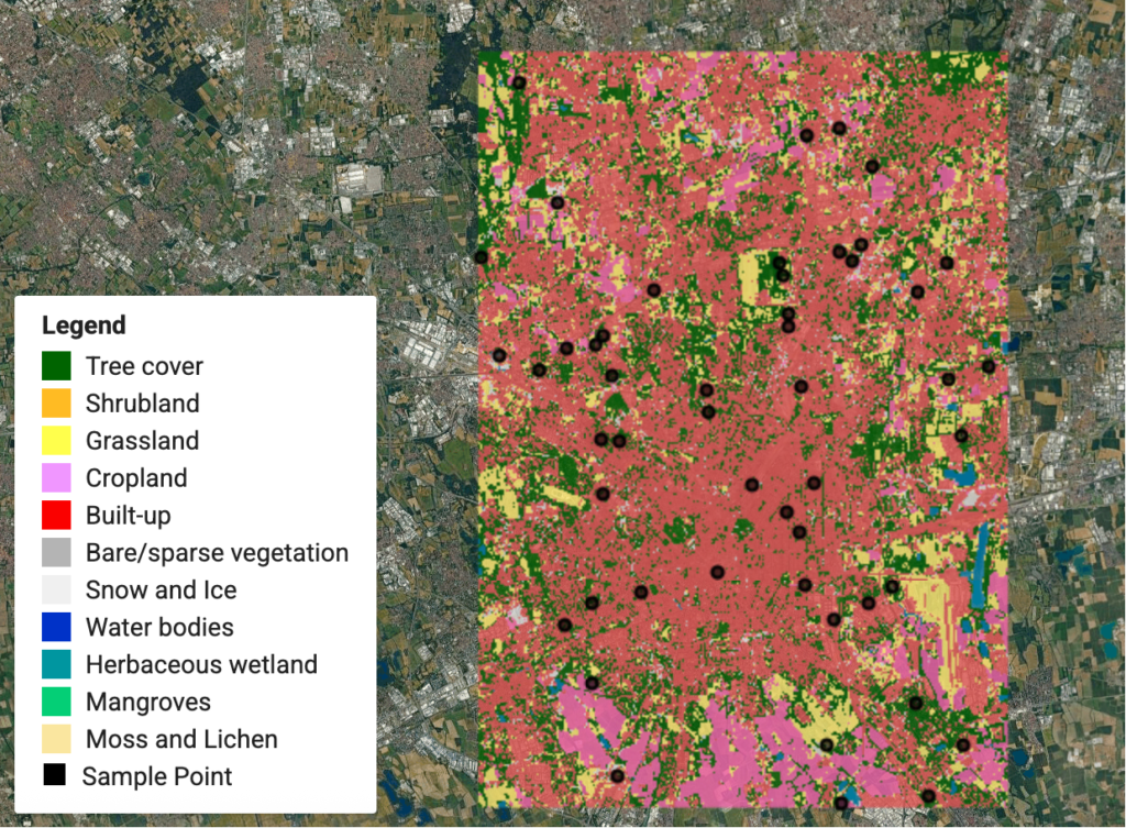
The fundamental purpose of an analytical map is to ask questions of spatial data. It may contain several competing classifications, intermediate calculations or layers that would be confusing in a public report. An accessibility researcher might inspect a street network, barriers, destination points and travel-distance outputs in separate combinations. The map functions as an interface for inquiry: where do unexpectedly high values occur, which locations need field checking and which model assumptions could explain an anomaly?
Analytical outputs are not automatically valid simply because they are generated by GIS software. Different input networks, catchment definitions, walking speeds and obstacle assumptions can produce different accessibility surfaces. A researcher should record those modelling choices rather than presenting a single colourful map as if it were a direct observation. The geography of the result depends on how the question was operationalised. A model of network distance is not a field survey of pedestrian experience, and a network connection does not prove that the route is comfortable, safe or open at all times.
The analytical map should preserve enough detail to audit calculations. Attribute tables, source geometry, alternative symbologies and visible outliers are valuable in this context. Temporary layers may be named by their processing stage, but final analytical records should use clear descriptions and store the variable, unit, spatial reference and date of the underlying dataset. An exploratory choropleth might show class breaks selected to expose variation, whereas a comparison across dates may require fixed breaks; this is an explicit analytical decision, not merely a change in palette.
A second obligation is to challenge the map’s support and resolution. The Office for National Statistics recommends standardised rates for area choropleths rather than raw totals and warns that mapping is not always the best way to compare a few geographic categories (ONS choropleth guidance). Similarly, the USGS explains why map projections differ in area and distance properties (USGS projection guidance). These sources reinforce a general methodological rule: a spatial visualisation must be designed around the statistical and geographic properties of the question. The GIS interface makes many options possible, but availability is not evidence of suitability.
When anomalies appear, analytical mapping should prompt verification rather than narrative closure. A sudden concentration of reported incidents may reflect a genuine hotspot, higher observation intensity, different reporting coverage or an incorrect spatial join. Visual inspection can help locate the problem, but cannot alone distinguish those explanations. That uncertainty should be resolved, or explicitly retained, before the result becomes a presentation figure.
A presentation map is a structured argument for a specific reader
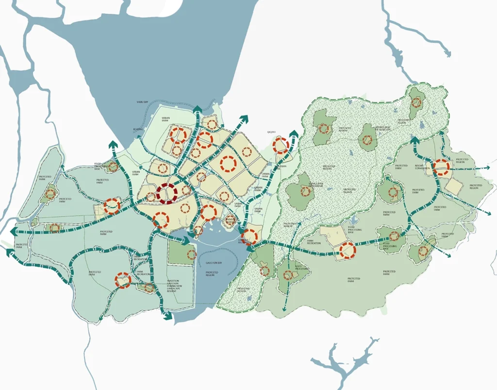
Presentation mapping is not the abandonment of analysis. It is the deliberate reduction of visual information so that a tested finding can be examined. The relevant question changes from “what could be happening here?” to “what can the available evidence support?” A journal figure, a municipal briefing and a studio presentation may use the same dataset but require different levels of annotation, explanatory text and technical detail. Their claims should remain compatible even when their graphic forms differ.
A presentation map needs a title that names the actual variable and geography. “Connectivity” is vague if the figure actually shows a particular network centrality metric. “Flood-prone area” may overstate evidence when the layer depicts only a scenario-based inundation model. A careful title separates observation, modelled output and proposal. A legend should explain the mapped quantity and units; a source line should make the evidence traceable; a note should disclose a major exclusion or assumption that affects interpretation.
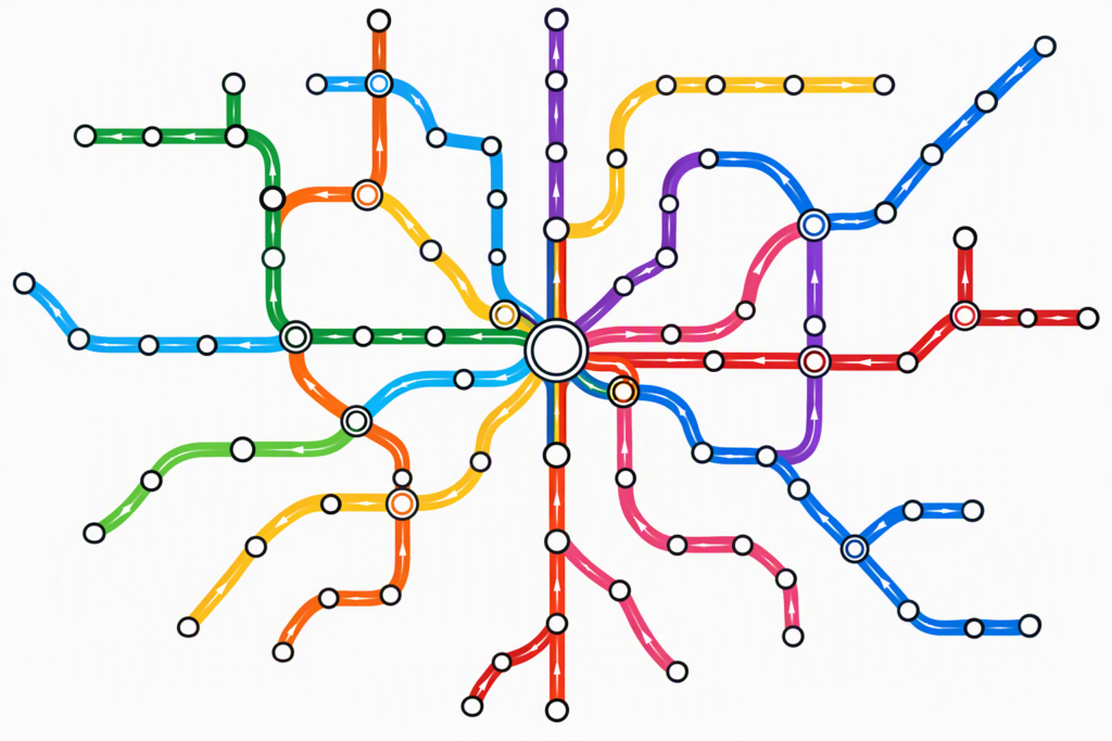
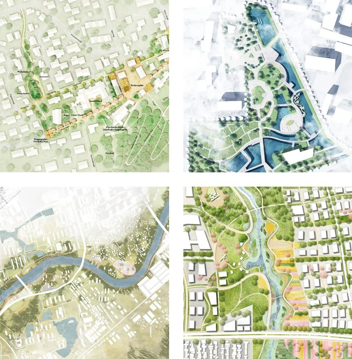
Graphic hierarchy then becomes an editorial method. The main dataset should dominate, contextual roads and buildings should recede, and the annotation should identify the key comparison without crowding it. Aileen Buckley’s discussion of cartographic principles explains how contrast, figure-ground relationships and proportion support map comprehension (Esri cartography guidance). The implication is not that every publication requires elaborate styling. A simple black-and-white building-footprint comparison can communicate more convincingly than a richly textured sheet when the research question concerns change in urban grain.
The presentation figure should also remain honest about what it omits. Cropping to a precinct may improve local legibility but remove neighbouring barriers. Generalising minor streets may improve a metropolitan figure but conceal micro-scale permeability. Such omissions can be defensible when they are consistent with the intended inference. They become problematic when the omitted information could reverse or materially qualify the stated conclusion. A locator inset, explanatory label or companion map can often restore the necessary context without sacrificing clarity.
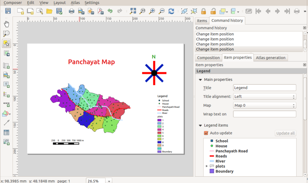
Finally, the figure must survive the publication medium. QGIS Print Layout can export to image, PDF and SVG and includes controls for map items, legends and labels (QGIS print layout documentation). A map designed at full-screen zoom may become unreadable when placed inside a two-column academic article. Presentation mapping therefore includes final-size testing, not merely visual approval inside the editing program.
The transformation must preserve measures, geography and uncertainty
A reliable translation from analytical to presentation map can be described as a sequence of accountable decisions. First, lock the analytical result: define the source dataset, variable, spatial unit, date range and processing method. Second, specify the audience and the single question the figure must answer. Third, remove extraneous visual layers while retaining enough geographic context to interpret the result. Fourth, redesign the legend and annotation so that a reader unfamiliar with the workflow can verify what is mapped. Finally, compare the publication image against the analytical source for unexpected changes.
This process also distinguishes a harmless visual refinement from a substantive analytical alteration. Reducing road stroke width usually changes hierarchy without changing the measured network. Reclassifying values, removing outliers, smoothing a raster or relocating points can change the evidence itself. Reclassifications may be legitimate, but they require explicit reasoning and sometimes renewed analysis. Treating these edits as mere graphic finishing creates a methodological blind spot. A map that looks cleaner after an undocumented change may be harder, not easier, to defend.
Take a hypothetical land-use change study comparing two survey years. A researcher might generate separate analytical maps to inspect classifications, boundary inconsistencies and missing parcels. A presentation pair should use comparable extents, a stable classification scheme and common graphic dimensions wherever the underlying data permit. If a land-use code was revised between surveys, the categories need harmonisation before they can be described as change. Photoshop or Illustrator can help align the panels, but cannot independently validate the correspondence of the classifications.
Similarly, a corridor accessibility map may be based on travel-time modelling, observation or self-reported perceptions. Each produces a different kind of evidence. A publication may show a striking gradient and include a representative photograph, but a photograph of a busy street does not prove the numerical model. Visual materials should support distinct claims and be identified by type. This distinction is especially important when proposed pedestrian interventions are shown on top of observed conditions: solid versus dashed lines, separate layers or explicit legend categories should keep scenario and reality apart.
Uncertainty should be represented proportionately. It is rarely useful to crowd every figure with an exhaustive methodological appendix, yet uncertainty that affects the interpretation belongs near the map. It might be a note stating that incomplete streets were excluded, a panel showing alternative assumptions, or a companion chart of confidence intervals. The goal is not to make every presentation complicated; it is to prevent apparent certainty from exceeding the evidence.
Use complementary maps and graphics instead of forcing one figure to do everything
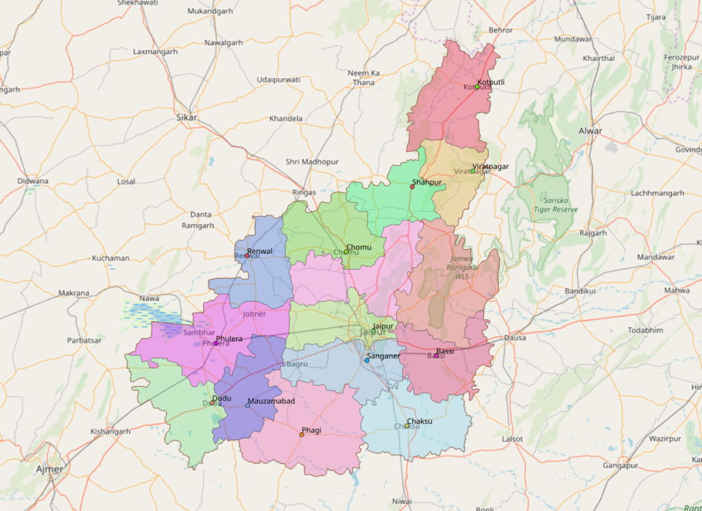
The map/chart decision deserves more attention than it often receives. The UK Office for National Statistics states that a bar chart can be clearer than a map when only a small number of geographic regions are compared, or when the geography adds little insight (ONS choropleth guidance). This is particularly relevant to urban reports that compare a few neighbourhoods, transit corridors or policy alternatives. A map is helpful for spatial relationships, but it is not automatically the clearest instrument for numerical ranking.
A well-designed research spread may therefore combine a locator map, an analytical thematic map and a compact statistical chart. Each component contributes a different kind of evidence. The locator establishes place, the thematic map reveals distribution, and the chart allows more precise value comparison. An accompanying photograph can document on-the-ground conditions but should not be used as a substitute for systematic observation. Integrating these representations is a stronger strategy than adding more variables to a single map until every graphic element becomes too small.
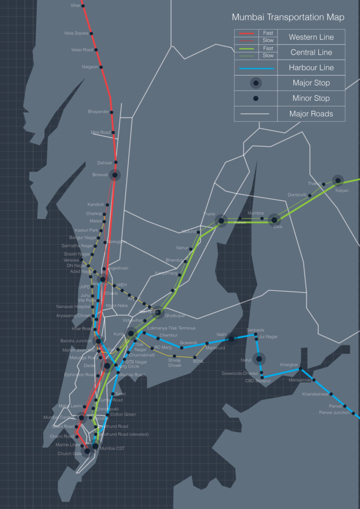
Scale-specific series are another valuable approach. A metropolitan map can show transit structure and peripheral growth; a district map can show walking networks and barriers; and a street-scale figure can examine frontages, crossings and public-space configuration. These maps should be related by consistent naming, sources and cartographic conventions. They should not be forced into identical symbol detail because the scale and analytical purpose differ. The USGS’s account of cartographic generalisation provides the conceptual justification for adapting displayed detail to scale (USGS cartographic representation).
For a practical example, consider investigating the relationship between urban heat and public space. One analytical figure might compare observed air-temperature readings, another model surface-temperature patterns, and a third map tree-canopy or impervious-cover distributions. Presenting these as the same variable would be misleading. A carefully framed multi-panel presentation can instead disclose which measurements are observations, which are remotely sensed indicators and which are plausible explanatory factors requiring further testing. This makes a stronger scientific argument than an apparently seamless but conceptually mixed heat map.
Complementary graphics also improve accessibility. A colour gradient may be hard to distinguish for some readers, while labelled values or an adjacent chart provide an alternative route into the evidence. W3C accessibility guidance cautions against using colour as the only carrier of information in covered digital content (W3C WCAG 2.2). Though the requirements are context-specific, the editorial principle is broadly useful: readers should not have to infer every conclusion from a subtle hue difference. Use text, consistent labels and alternative representations where they materially improve interpretation.

A review protocol can keep both map types academically defensible
The practical distinction can be institutionalised through a short review protocol. For the analytical map, ask whether the variable is defined, the spatial unit is appropriate, the input sources are recorded, and plausible alternative explanations have been considered. For the presentation map, ask whether the title matches the measure, the visual hierarchy is intelligible, the map includes necessary context, and the output is readable at publication size. Both should be checked for source and date consistency. These tests evaluate different risks but share the same standard of evidence.
File organisation should reflect that distinction. Keep analytical work in versioned GIS projects with input data and processing documentation; export stable outputs for the publication stage; and preserve editable Illustrator or Photoshop files as downstream communication assets. QGIS documentation makes clear that PDF and SVG export settings affect whether output is vector-based or rasterised (QGIS export documentation). An attractive editable file is not necessarily a complete record of the GIS analysis. Conversely, an annotated GIS project is not necessarily a reader-ready figure.
Peer review can expose overlooked mismatches. Ask one reviewer to inspect the data and method and another to interpret the final map without explanation. If the second reviewer identifies a pattern that the first reviewer knows the analysis cannot support, the map has an evidential communication problem. Revise the claim, graphic encoding or supporting note accordingly. Treat such feedback as a diagnostic instrument, not a referendum on aesthetic taste.
In teaching and practice, this dual-map approach can make urban studies more transparent. Students can submit an analytical figure showing intermediate testing alongside a refined final plate. Planning offices can retain a detailed working map while issuing a public-facing version with clearer legend and source. Research teams can track how a model output changes as it becomes a journal illustration. The benefit is not only visual quality; it is a visible chain of reasoning from data to decision.

Conclusion
An analytical map explores spatial evidence; a presentation map communicates a defined and defensible interpretation. The two overlap, but they should not be treated as sequential aesthetic states of the same image. Valid measures, consistent geography and acknowledged uncertainty must survive the translation. Professional cartographic principles, official statistical guidance and careful GIS export practice provide practical safeguards (Esri cartography guidance) (ONS choropleth guidance) (QGIS export documentation). When a research team designs both products deliberately, the resulting urban maps become easier to audit, teach, debate and use responsibly.
References / Further Reading
- Esri, Primary Design Principles for Cartography
- UK Office for National Statistics, Choropleth Maps
- QGIS Documentation 3.44, Overview of the Print Layout
- QGIS Documentation 3.44, Creating an Output
- US Geological Survey, How Are Different Map Projections Used?
- US Geological Survey, Cartographic Representation
- World Wide Web Consortium, Web Content Accessibility Guidelines 2.2